FLUX and pathways viewER
FLUX and pathways viewER
Fluxer can compute and visualize different flux graphs of genome-scale metabolic models by performing Flux Balance Analysis (FBA) and analyzing the resulting fluxes. Users may explore any of the models already available in the website or upload their own models in SBML format.
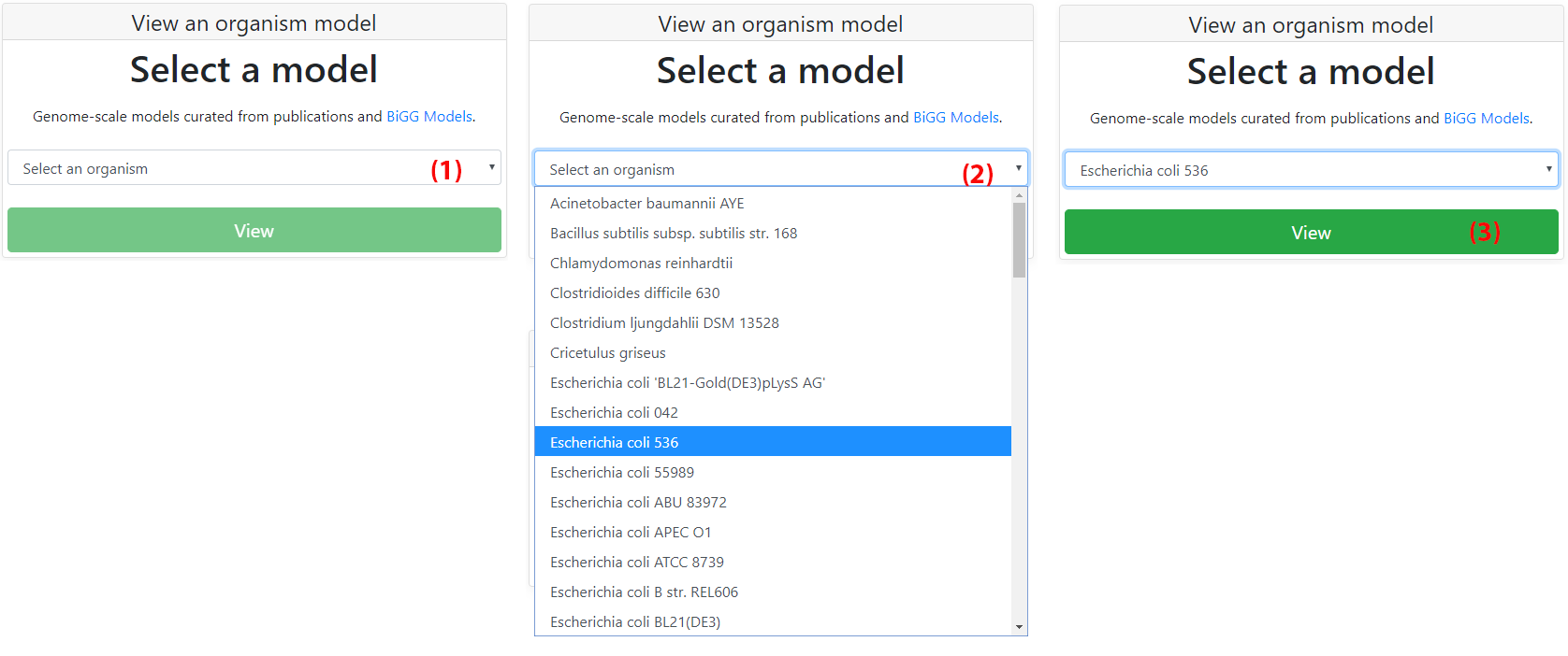
Fluxer includes more than 100 pre-loaded models for any user to explore. The drop down menu (1) on the home page lists all the available curated models. Any model from the menu can be visualized with the tool. Clicking on "View" (3) will then load the model and the visualization interface will be shown with the corresponding spanning tree.
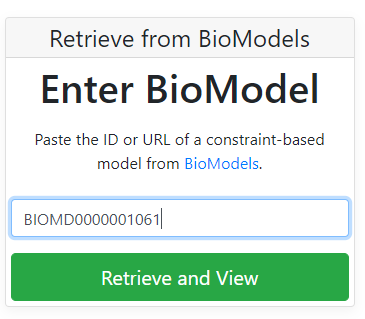
BioModels contains a collection of mathematical models of various biological systems. Fluxer can directly retrieve and compute graphs of constraint-based models from BioModels. To retrieve a model, copy either the 'Model Identifier' or model webpage URL and paste it into the 'Enter BioModel' textbox on the Fluxer homepage. Then click on the 'Retrieve and View' button and the system will retrieve and generate the flux graph. This page lists all the constraint-based mdoels available in BioModels.
Any model following the SBML specification can be analyzed and visualized with Fluxer. To upload a model, click on the "Choose File" button from Fluxer's home page (1).
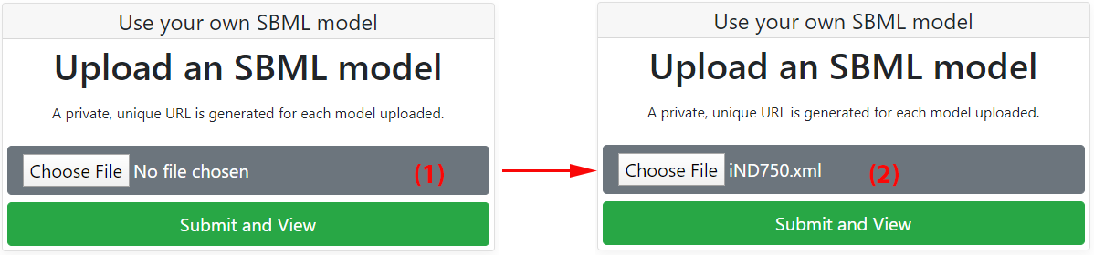
Next, select the desired SBML input file from a folder in the local computer. The file name and extension should be visible on the grey box once the file is selected for uploading (2). Finally, click on the green "Submit and View" button to upload and analyze the model with Fluxer. If the input file format is not recognized by Fluxer, an error message will appear after submitting the file. Once the model has successfully been loaded into the server, a private and unique URL for the model will be generated and the model visualization page will be shown. The URL for the model visualization page is shown in your browser, and can be saved and shared for future access to the model. By default, the spanning tree for the model is shown.
The graph visualization interface includes a main central area for the graph display and two collapsible side cards with interactive graph options and information.
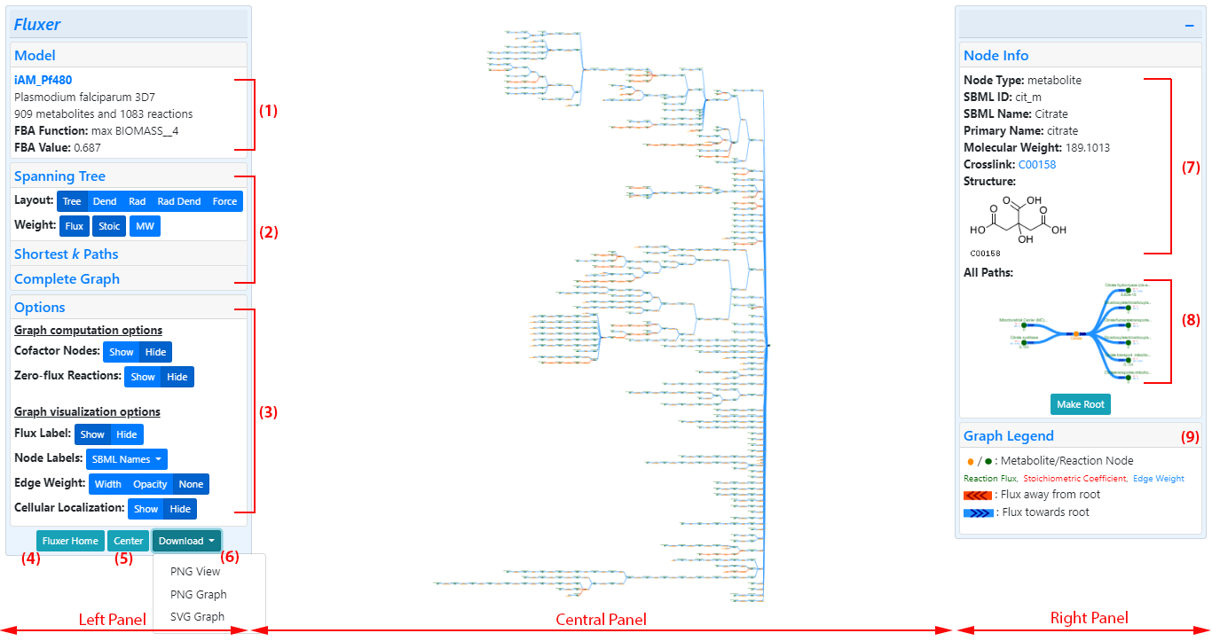
The collapsible card on the left includes sections for the model summary, graph computations and layouts, and graph options.
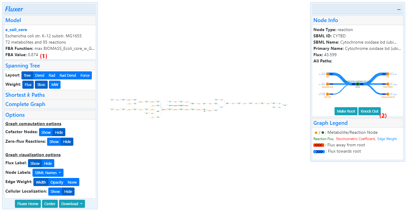
Model summaryThe model section (1) contains the current model name obtained from the SBML file including a hyperlink to the publication or BiGG database entry. The name of the organism and particular strain is also displayed, if available. The next lines in the section summarize the number of metabolites and reactions, the FBA objective function, and its optimized value.
Fluxer graphsEach graph section (2) specifies a different graph computation that Fluxer can perform. Buttons to control the layouts for each graph are included in each section, as well as buttons to specify the weight computation for the edges, if applicable. Clicking on a graph section collapses the other graph sections and refreshes the central graph panel to display the corresponding graph selected. The visualization options for the Spanning Tree, k-Shortest Paths and Complete graphs are explained in detail below. The figure below shows the Spanning Tree section expanded and including the layout and weight controlling buttons for the graph.
Selecting graph computation and visualization optionsThe options section (3) contains buttons to control the computation and visualization for all graphs. This section is explained in detail below.
Navigating to Fluxer homepageClicking on the Fluxer home button (4) opens Fluxer's homepage in a new browser tab.
Centering the graphAs the name suggests, the center button (5) re-scales and centers the graph in the browser window.
Downloading graph images and metabolic modelThe download button (6) on the left card allows users to download the current view or current graph in PNG format.The current graph can also be downloaded in SVG format. The metabolic model can be downloaded in SBML and graphML formats. This is particularly useful when users want to download a merged model.
The central panel contains the canvas on which the interactive graphs are rendered. The graph visualization can be zoomed in and out using the mouse scroll wheel and panned by dragging the graph. Clicking on a reaction or metabolite node opens the right panel and displays detailed information about that node.
Right panelClicking on any node in the graph or the "+" button on the top right corner opens the right card and shows information about the last node clicked, either a reaction or a metabolite. Upon loading the graph, the default node information displayed is for the root node.
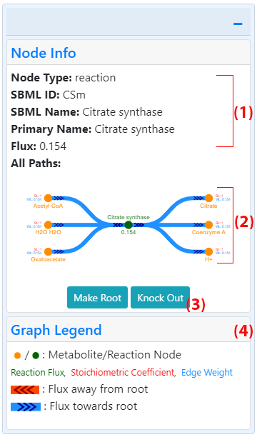
For both types of node, the node type (metabolite or reaction), complete SBML names, SBML IDs, primary name, crosslink (when available) and All Paths graph are displayed in the right card. The crosslink shows the entity ID linked to an appropriate database with more information about the metabolite or reaction. Some metabolites cross-reference to KEGG and thus the KEGG compound ID is displayed in this case. The metabolites with available KEGG IDs also display their molecular structure within the node information panel. The crosslinked KEGG ID and molecular structure for citrate are shown in the figure showing the full fluxer interface. When information is displayed for a reaction node, the panel displays the reaction flux computed in the FBA optimization.
All paths graphThe All Paths graph (8 in figure showing interface, 2 in figure showing right card) displays all the nodes connected to the selected node for which information is being displayed. Reaction nodes show all the metabolites involved in that reaction. Metabolite nodes show all the reactions that the selected metabolite is involved in. Unlike the larger central panel graph, co-factor and zero-flux reactions are always included in this graph. Users can also zoom in and out of this graph, pan it by dragging the mouse, and click on any node to show more information about it. In addition to the node labels with the format selected from the general graph options (3), the nodes in this graph display the stoichiometric coefficient (St.) and the weight (Wt.). The color legend (9 in figure showing interface, 4 in figure showing right card) explains which colors correspond to each label.
Graph legendThe graph legend section (9 in figure showing interface, 4 in figure showing right card) contains descriptions of the node, edge, text, and arrow colors and shapes. In the case of the k-shortest paths graph, the legend shows the color key mapping used to represent each different path. The legend is displayed in the interface image below for the k-shortest paths graph.
Simulating knockoutsThe right card includes a "Knock Out" button (3 in figure showing interface) when a reaction node is displayed. Clicking this button adds the current reaction to a list of knocked-out reactions. The simulation of knockouts is explained in detail below.
The spanning tree is the default graph displayed after a model has been loaded. The panel on the left of the interface allows the user to change the type of flux graph to visualize and to select different visualization options.
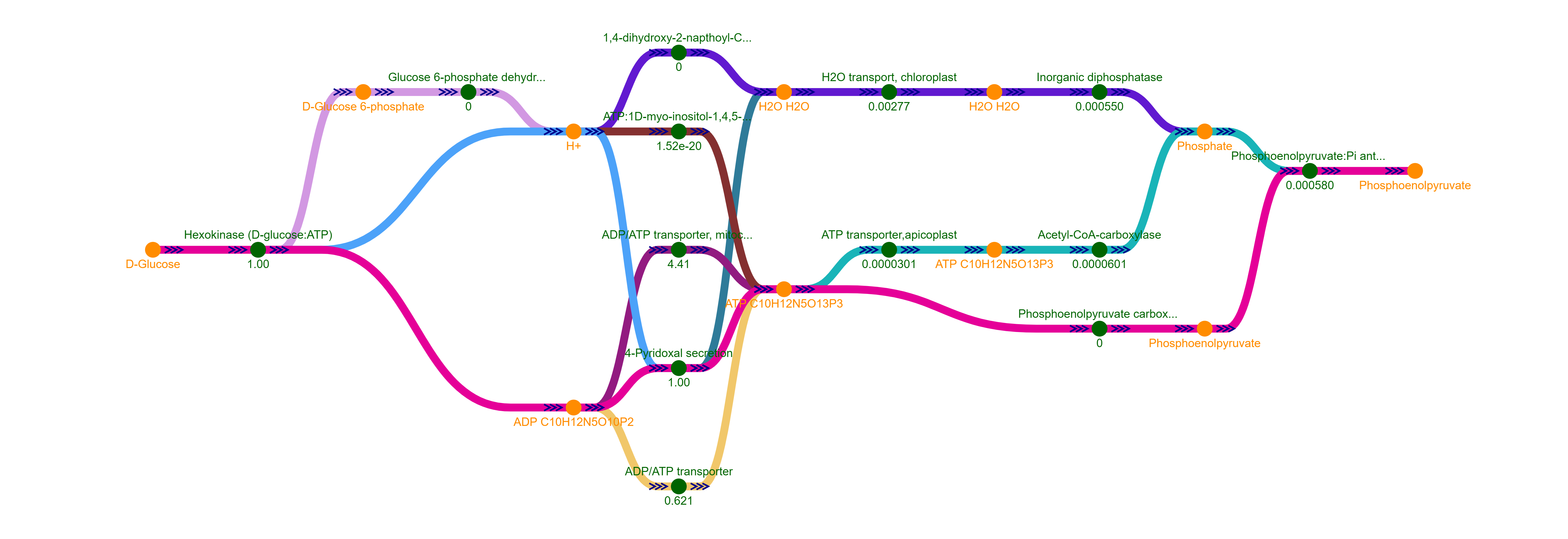
The spanning tree shows the most important connections between all reactions and metabolites towards a given root node. Fluxer sets the objective function reaction as the root node by default, but the user can select any other reaction or metabolite as root. The tree is built iteratively starting from the root node and adding the edge with the highest weight that connects a current node in the tree with a node not yet present in the tree, giving preference to the closest edge for similar weights. Weights can be selected to be any combination of flux, stoichiometry coefficient, and molecular weights. When flux is the only weight used, the generated tree is a "flux" spanning tree, as shown in the figure below. Blue edges represent fluxes moving towards the root while red edges represent fluxes moving away from the root.
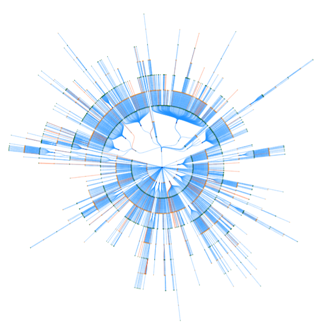
An example of a spanning tree for Plasmodium falciparum is shown below. (A) Full spanning tree. Branch within red square is zoomed in (B). Green nodes represent reactions and yellow nodes represent metabolites. The numbers below the reaction nodes indicates the reaction flux. Arrow heads indicate the direction of the flux going out of the root node (red edges) or coming in the root node (blue edges). The spanning tree uses reaction fluxes and stoichiometric coefficients on edge weights, and excludes cofactor metabolites and zero-flux reactions
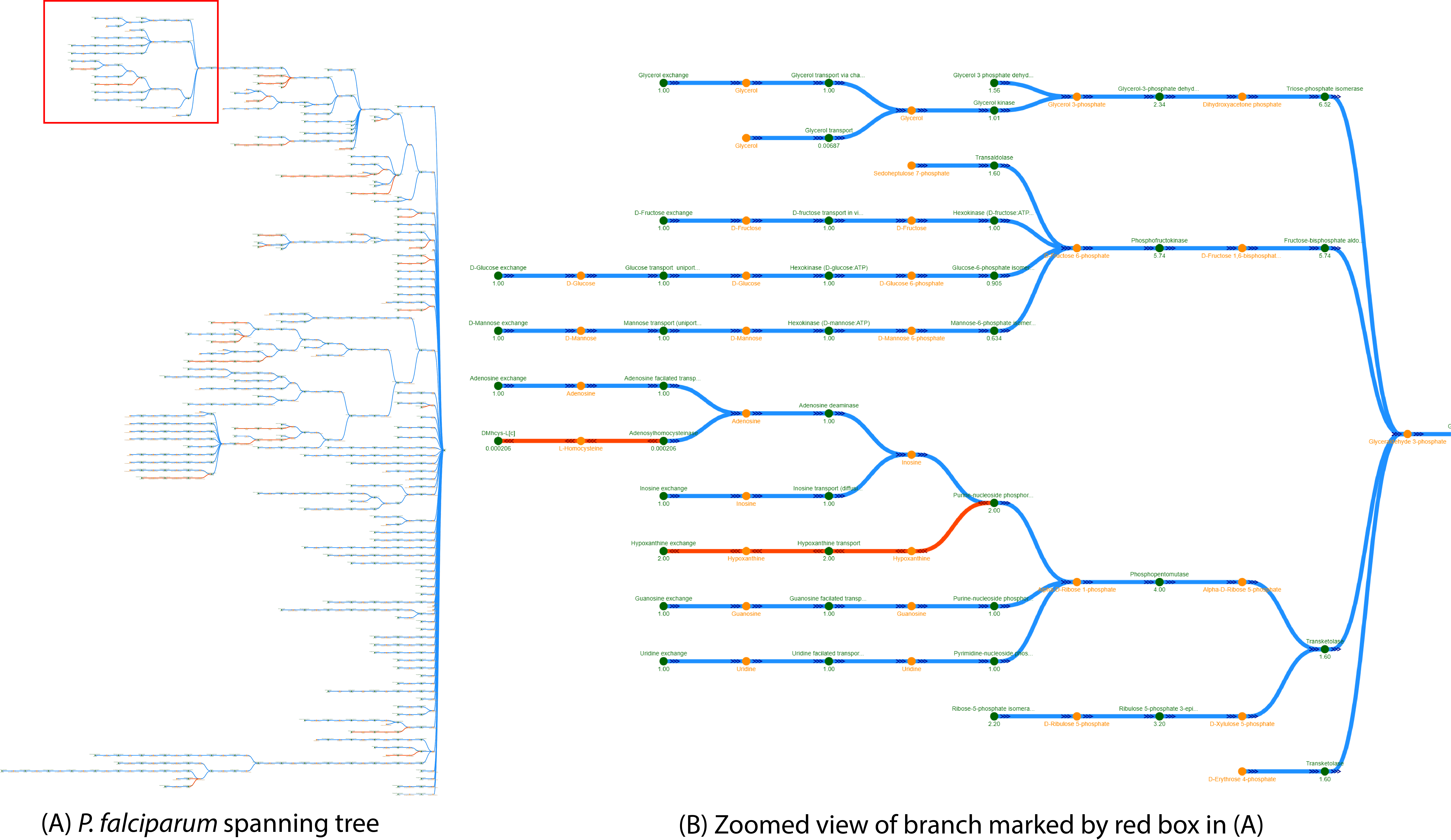
By default, the spanning flux tree is generated using the reaction flux and stoichiometric coefficients as the link weights. To change the weights in the tree links, users can click the corresponding buttons on the panel shown as "Flux", "Stoichiometric Coefficient", and "MW" (Molecular weight). The root node is the objective function reaction by default. This can be changed by clicking on any node and clicking the "Make Root" button from the panel that appears on the right. The adjacent button, "Reset tree", can be used to change the tree back to the default root (objective function reaction node). The tree can also be viewed with a Dendrogram, Radial, or Force layouts by clicking on the corresponding buttons in the left panel.
Fluxer can compute the k-shortest paths between a given source and target metabolite or reaction. The algorithm first finds the shortest path between the source and target nodes using the same method that for the spanning tree algorithm. Then, the algorithm iteratively removes every edge in the shortest paths found so far and then the same shortest path algorithm is applied. Fluxer can compute either the best k shortest paths (optimal) or the first k shortest paths found (faster).
The example below shows the k=5 paths between D-Glucose and Biomass in Plasmodium falciparum. (1) The best and first paths reload buttons (re)calculate the k-paths graph using the current selected settings. (2) The dropdown lists allow to change the source and target nodes. (3) Either a dagre or force layout can be selected to display the graph. (4) Buttons to control the weight on the graph used to calculate the shortest flux paths. (5) Detailed information about the clicked node (D-Fructose 1,6-bisphosphate) is shown on the right panel. (6) Mini-graph showing the neighbors of clicked node. (7) Graph legend describing the colors of the nodes and for each kth path.
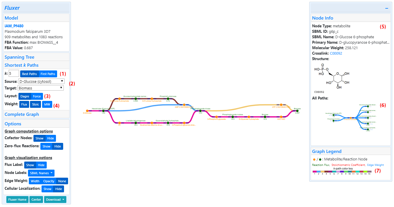
Clicking on the "Shortest k Paths" link on the left panel generates the shortest path between the source target nodes. As in the spanning tree, the default target is the objective function reaction node. The name of the nodes in the dropdown are sorted alphabetically and includes the suffix indicating which cellular location the metabolite or reaction is located in (cytoplasm, extracellular, etc.). The number of paths to compute is input in the "k" box. Clicking on the "Best Paths" or "First Paths" button computes and displays the graph. The weight used for the links is the reaction flux and stoichiometric coefficient by default, but the user can change it by clicking on the buttons indicated with the "Weight" label. The visualization can be switched to a force layout by clicking on the corresponding button.
It is particularly useful to hide the
co-factor nodes when generating this graph for more biologically feasible solutions as shown below:
a. Excluding Cofactors

The complete graph displays all the metabolite and reaction nodes in the model. It can be visualized as a graph with a force layout. In addition, it can be visualized as a tree with a breadth-first traversal from a selected root node in a tree or radial layout, duplicating metabolites and reactions as necessary. Fluxer can also generate the complete graph in SBML layout if coordinates have been provided using SBML layouts extension in the SBML file.
The example below shows the interface with the complete metabolic network of Plasmodium falciparum with a force layout. The labels are hidden, but the cofactor and zero-flux reactions are included in the graph shown.
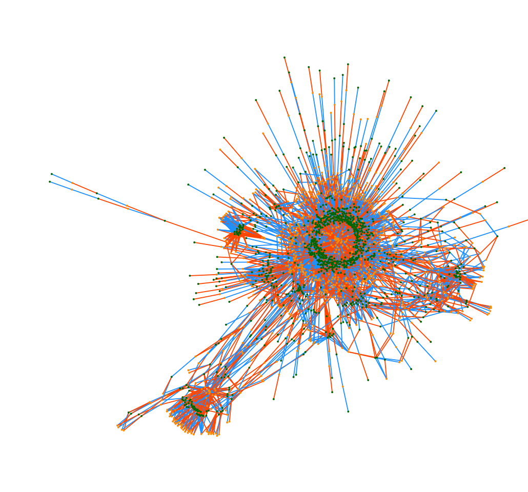
Clicking on the "Complete Graph" link from the left panel generates the complete metabolic network graph. The force layout visualization is displayed by default. The complete graph can also be visualized with a tree layout.
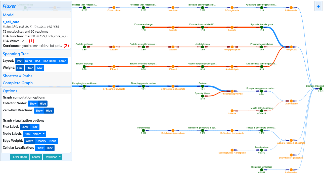
Fluxer allows users to perform any number of reaction knockouts. Once a reaction is knocked-out, a new FBA is simulated and the current graph is recomputed based on the new flux values. The figure below shows the effects of knocking-out a reaction in the E. coli core model. Cytochrome oxidases are involved in the aerobic respiration pathways. As expected, knocking-out one of these oxidases activates the fermentation pathways in E. coli. This knockout also results in a reduction in growth rate, as shown with the decrease of biomass objective value after the knockout.
When building genome-scale metabolic models, users may need to merge and curate several draft
reconstructions. Further, comparing draft reconstructions can provide information about which metabolic
components are unique to each draft reconstruction and common between all. Similarly, comparing validated
genome-scale metabolic models of different organisms can help identify metabolic pathways that make each
model unique and identify the pathways that enable both organisms to have similar metabolic phenotypes.
Fluxer uses the python package mergem to merge two or
more genome-scale metabolic models.
Results from mergem are used to visualize the components unique to each model and common between all
input models using different colors in the Fluxer graphs, as explained below.
Metabolites and reactions may also be translated from the identifiers used in one of the supported
databases to those of another. Translation may be performed standalone or as part of the merging process.
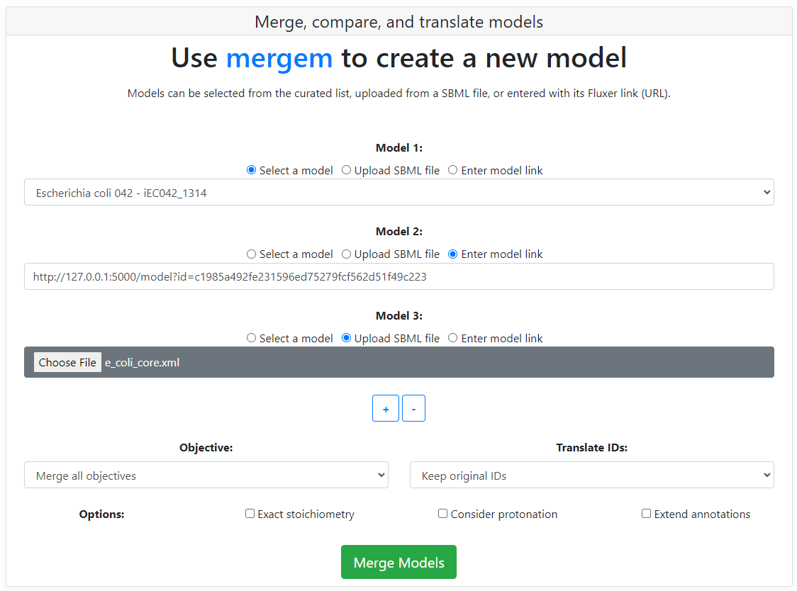
The user can choose from one of the curated models in the dropdown, upload new model files (in SBML format), or enter Fluxer model links.
The objective function for the merged model can be set from one of the input models or be combined in a reaction that merges all the objective reactions from all the input models. The dropdown located below the input models is used to select the type of objective desired.
Metabolite and reaction IDs can be translated during merging multiple models or for a single model. The target database ID system can be selected from the dropdown. For translating a single model, remove the second model input by clicking the '-' button.
By default, reactions are merged when they have both a similar set of reactants and a similar set of products, without comparing their stoichiometry. To merge reactions only when they have the same exact stoichiometry in their reactants and products, select the "Exact stoichiometry" checkbox prior to merging the models.
By default, reactions are compared ignoring the hydrogen and proton metabolites. To consider also the hydrogen and proton metabolites when comparing reactions, select the "Consider protonation" checkbox prior to merging the models.
Metabolite and reaction annotations are merged from all input models. In addition, these annotations can be extended in the merged model using the mergem database. Select the "Extend annotations" checkbox for extending the annotations using the mergem dabase.
After generating the merged model, the Fluxer graph interface loads the merged model graph in a special
view to compare models. In this view, the metabolites and reactions unique to each
model are shown with a different color each and the metabolites and reactions common between all models
are shown in green:
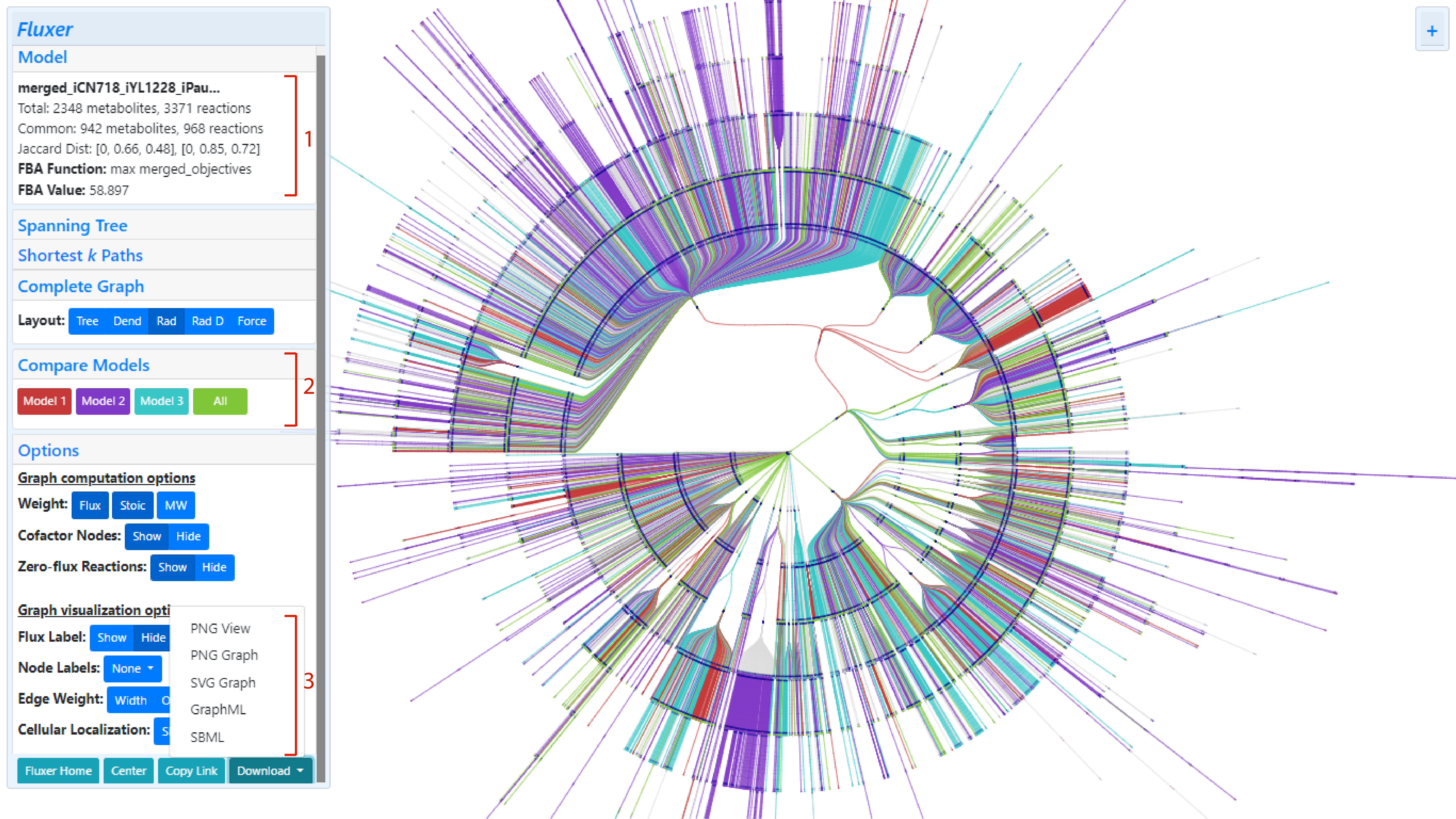
Graphs of merged models can be viewed with the standard Fluxer colors by clicling and collapsing the "Compare Models" card on the
left panel.
The model summary card also includes the total number of metabolites and reactions in the resultant merged model as well as the number of metabolites and reactions merged.
The merged metabolic model can be downloaded in SBML and graphML formats using the "Download" button on the left panel in the visualization interface.
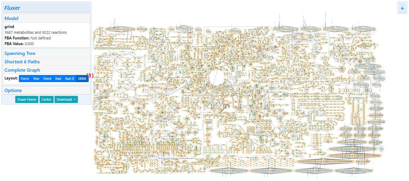
Fluxer can display the complete graph using the layout stored in the models. For this, a model needs to
use the SBML layout extension format. If a SBML layout is detected in the model, a button (1) for displaying
the complete graph with this layout is deplayed. An example of this type of layout is shown below for
ReconMap-2.01.
The left panel on the visualization interface contains the following options to customize how the flux graph is computed and displayed.
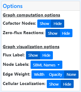
The user can toggle the visibility of the flux labels shown below the reaction nodes.
The dropdown list can be used to select which labels to display in the nodes. The user can select between labels generated with either SBML IDs, SBML names, primary names, or no labels. The first two options are derived from the SBML model. Primary names are generated from the best names found on different databases. None hides all node labels from the graph.
The weights on the links can be visually displayed as the edge width or as the opacity of the edge color. By default, no weights are used for the edge.
Small molecules (like water, carbon dioxide, etc.) and cofactor metabolites (such as ATP, NADPH, etc.) can be excluded from the graph visualizations.
Reactions carrying a flux of 0 mmol/(gDCW * h) can be excluded from the graph to visualize only those reactions that participate in the objective function optimization.
The cellular compartment (cytoplasm, mitochondria, etc.) in which the metabolite is localized can be displayed next to the node labels.
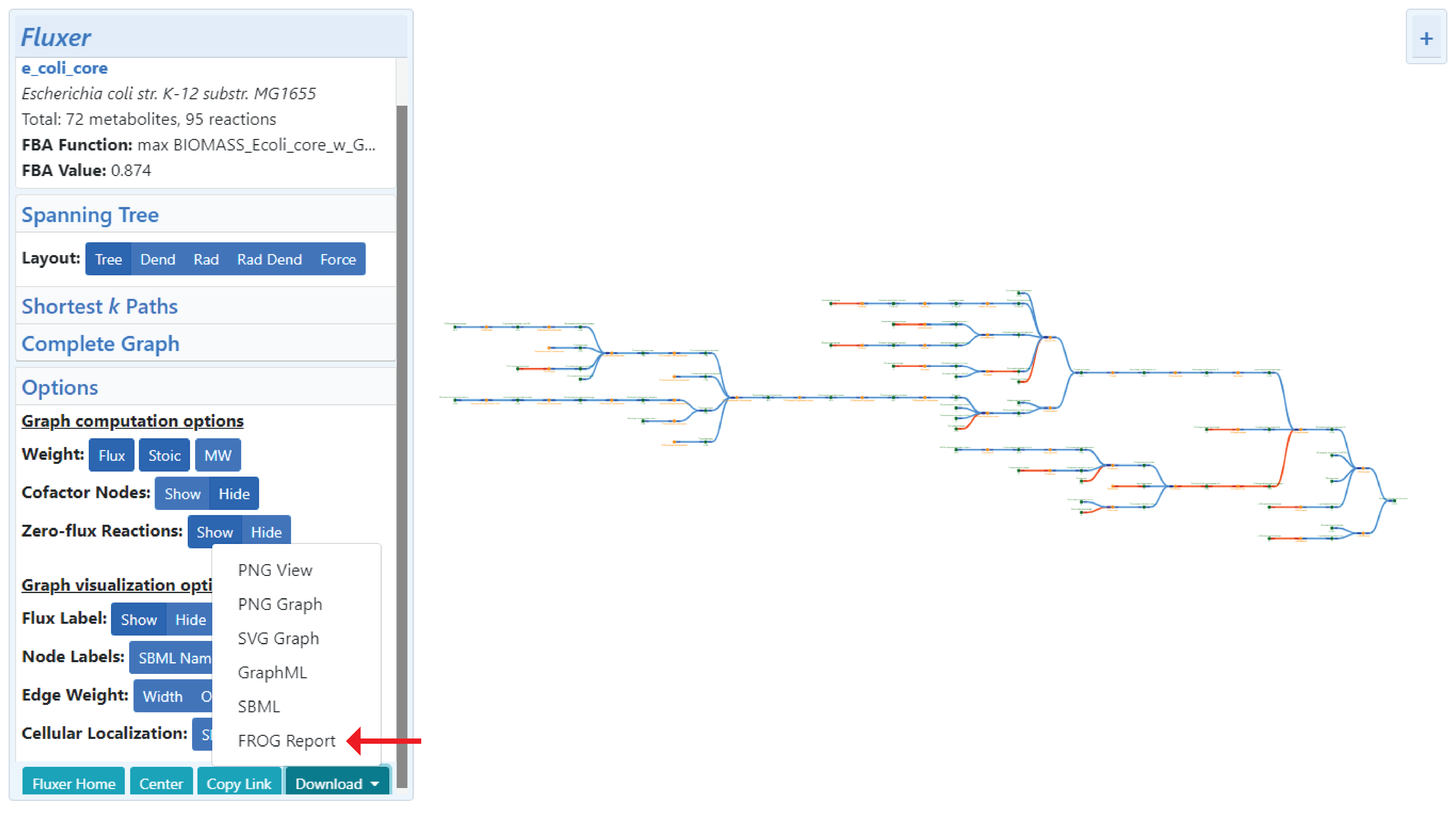
A FROG report is a numerically reproducible reference dataset that aids in the assessment of the reproducibility and curation of a genome-scale metabolic model. The report comprises of the following list of results: